Teaching Blar to Give Better Code Reviews: How We Built Our Text-Based Recommender
30-04-2025
Teaching Blar to Give Better Code Reviews: How We Built Our Text-Based Recommender
The code, idea, and concepts were all developed by Juan Vargas, one of our engineers at Blar.
Check out his:
LinkedIn: Juan Vargas
GitHub: v4rgas
I’m just the greedy CEO who wrote the article and stole the credit 🤑
The context
Blar is an AI agent that helps developers review their pull requests. Our long-term goal is to make Blar as smart and capable as a senior engineer within your organisation. But to create a senior, you have to start learning not just from your wins, but most importantly, from your mistakes.
One of the best ways to learn is through feedback — positive and negative interactions. That’s how we humans learn¹: by having a reward system that makes us feel good when we do something right, and not so good when we mess up. So, how can we build something similar for our Agent?
Recommender Systems
Recommender systems are everywhere — all around us. From video suggestions on YouTube and Netflix to product recommendations while shopping online, there’s always a recommender system working behind the scenes. These systems learn from your interactions and adapt to give you the best possible experience.
Recommender systems might feel like magic, but it’s really science… data science. They are built by observing what you like and what you ignore, using that data to predict what you might want next.
Let’s dive into the basics of how recommender systems work:
At their core, most recommender systems rely on two key approaches:
Collaborative filtering: This method learns from the behavior of users. If users similar to you liked something, chances are you might like it too. It’s like when your friends recommend a movie because you all have similar taste.
Content-based filtering: Here, the system looks at the properties of the items themselves. If you liked a sci-fi movie, it might suggest another sci-fi movie — because it knows the genre, director, or actors match your previous favorites.

At the end of the day, a recommender system is just trying to answer one question: What’s the next best thing I can show you that you’ll love? (or activate your neurons)

What does any of this have to do with Pull Request comments?
At first glance, it might feel like pull request comments and Netflix recommendations live in two completely different universes. But under the hood, it’s the same core idea: learning from interactions to make better suggestions.
Every time Blar leaves a comment on a pull request — whether it’s spotting a bug, suggesting a refactor, or flagging a code smell — we ask for simple feedback: just a thumbs up( 👍) or a thumbs down( 👎).
This tiny signal tells us a lot. A thumbs up means we were helpful (think dopamine). A thumbs down means we missed the mark and the user didn’t like our comment (think of it like a small pain signal).
But here’s the challenge: pull request comments come in all shapes and forms. How do we know what type of comment the user didn’t like? Was it a suggestion about a bug? About null handling? About user validation?
This was the key question that motivated us: are there specific types of comments that users consistently prefer — or dislike?
After talking to some of our users, a pattern started to emerge. They often said things like: “We don’t like when you flag null values,” or “Input validation issues aren’t really helpful for us.”
Understanding these preferences was the first step toward making Blar smarter — and more aligned with how your team thinks about code quality.
How to clasify “types” of comments.
Saying that our users don’t like “null values” comments is one thing — but how do we actually find which comments are about “null values”?
One simple alternative would be to just search for keywords like “null” or “value” inside the comment. But a much better way is to use embeddings( in this article, we go into detail)
Embeddings help us capture semantic similarities between texts. That means two comments that are roughly about the same topic should end up close together, i.e. they’ll have a small cosine distance.
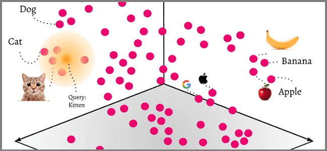
To generate embeddings, we just use a pre-trained in this case, Open AI’s embeddings.
Awesome. Now we have a way to understand if two comments are talking about the same thing.
But that leads us to a second question: what’s a suitable distance to say these two comments are of the same type?
For this, we turned our heads to clustering.
Clustering
Clustering is the idea of grouping similar things together without knowing how many groups there are or what they should look like. In our case, we wanted to group similar comments and discover the “natural topics” that Blar was commenting on.
There are many different methods of clustering, but for this example, we’ll use k-means, a classic and simple approach.
And just like that, we generated our clusters (the magic of sklearn, everyone ✨).
To visualise these clusters, we can use techniques like PCA (Principal Component Analysis), which is a dimensionality reduction method that helps us squash high-dimensional data (like 300 dimensions) down into something we can actually plot (like 2D or 3D).
We’re getting there.
But if you look closely at the code, you’ll notice we chose n_clusters=11².
Why 11 and not 10 or 12?
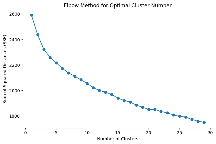
We used a technique called the “elbow method” to figure this out.
The idea is simple: you plot the number of clusters against the “error” (sum of squared distances), and pick the point where adding more clusters stops giving you a big improvement, where the curve bends like an elbow.
Here’s a rough version of the code we used:
Recommendation
Now that we have our clusters, we can finally generate real recommendations from them.
For this, we used collaborative filtering: based on what users from your company like (👍) or dislike (👎), we prioritize the types of issues that land in each cluster.
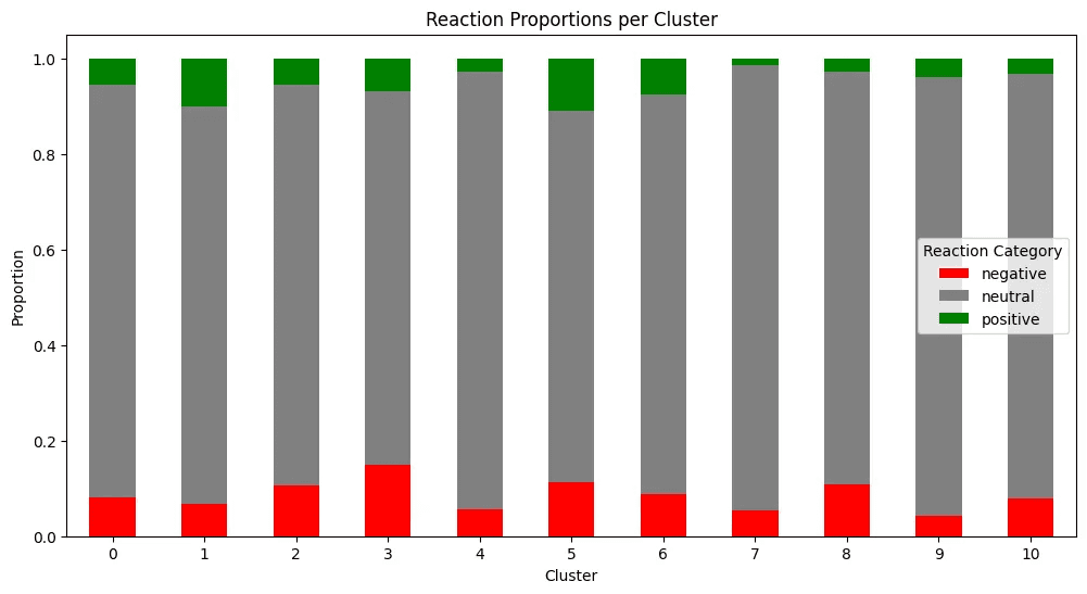
When we analyze feedback across clusters, we find that some, like Cluster 5, drive a lot of engagement, positive or negative. Others, like Cluster 7, tend to receive mostly dislikes or no interaction at all.
To decide which clusters to recommend from, we apply a simple rule: for each cluster, we compute a smoothed like ratio using the formula:
(likes + 20) / (total + 10)
This smoothing prevents a small number of votes from skewing the outcome too much. If the ratio is greater than 0.6, we recommend content from that cluster. If it falls below, we still recommend it 20% of the time to continue exploring potentially overlooked clusters.
This approach helps us prioritize high-quality clusters while still learning from the under-engaged ones.
A simple implementation looks like this:
And the __should_recommend function is a simple proportion-based logic:
That’s it! You now have your own recommender system based on text.
Warnings ⚠️
When dealing with embeddings — and data in general — you have to make sure you’re capturing the right information.
To explain what I mean:
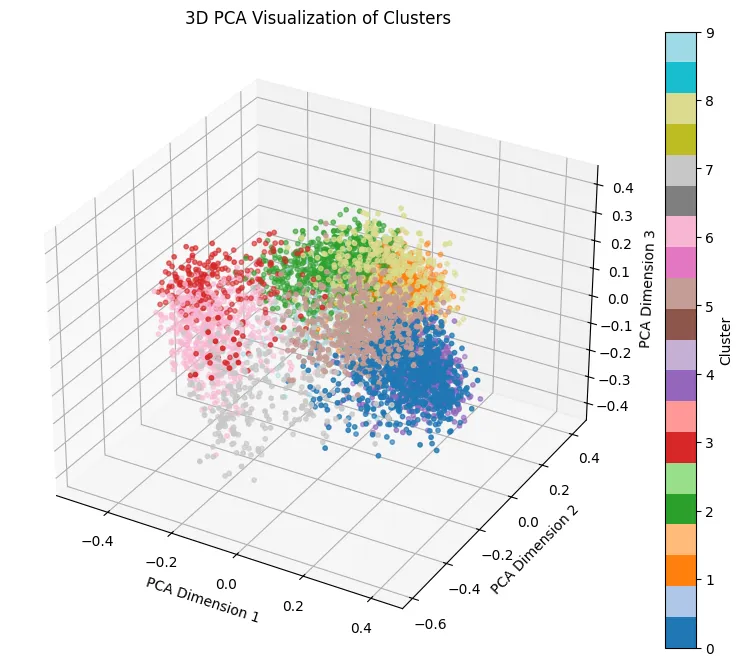
Our first approach at embedding the issues (without any sanitization) gave us this distribution across companies:
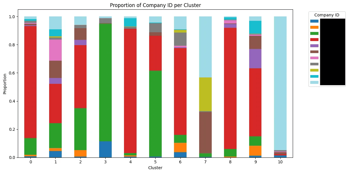
As you can see, the distribution was far from homogeneous.
For example, Cluster 10 was clearly dominated by a single company (light blue); instead of being about a real topic like “null values”.
Why did this happen?
When Blar suggests an improvement, it often includes:
Code snippets
Variable names
Business logic
These elements are highly specific to each company.
So when we embedded the issue, we weren’t capturing the topic — we were accidentally capturing company-specific fingerprints.
That’s not what we wanted.
🛠️ How we fixed it
To solve this, we sanitized the data:
We replaced any code snippets with a
<code>token.We replaced variables with a
<variable>token.
This way, the embeddings would focus only on the real semantic meaning of the comments, not the irrelevant, company-specific details.
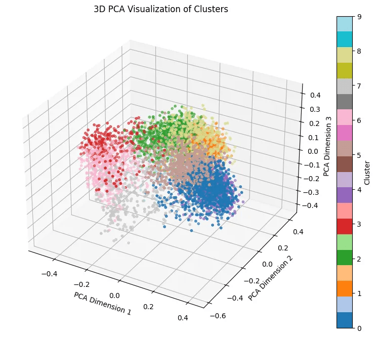
After sanitizing, we re-ran the clustering, and now the distributions looked like this:
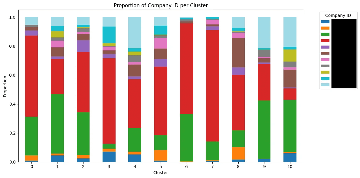
Much better — now the clusters are far more balanced across companies, meaning we’re finally capturing true topics instead of leaking company identity into the embeddings.
Extremely oversimplified and I’m not in any way whatsoever qualified to give a more profound answer.
You’ll also notice a random_state=42, but that’s because 42 is the answer to life, the universe and everything.
We help teams regain control of their codebase, ship faster, and stay ahead of technical challenges. If technical debt is slowing you down, let’s talk.
LinkedIn: Jose Dominguez
X: @LePeppManu
Blar: blar.io
Substack: Blar News
Thanks for reading!